LIME user manual
Note
This document can be read as a text file, but the markup format makes that a little annoying. The *.rst files are intended as sources for eventual HTML pages. The latter can be built via the command ‘make doc’. The resulting start page can be found at doc/_html/index.html. The HTML version is also available online at the https://readthedocs.org/projects/lime/ website. The present file is only intended to be a summary.
Introduction
Disclaimer
We, the authors and maintainers of LIME, do not guarantee that results given by LIME are correct, nor can we be held responsible for erroneous results. We do not claim that LIME is perfect or free of bugs and therefore the user should always take utmost care when drawing scientific conclusions based on results obtained with LIME. It is very important that the user performs tests and sanity checks whenever working with the LIME code to make sure that the results are reasonable and reliable. In particular, care needs to be taken when extending the runtime parameters into regimes for which the code was not designed.
The LIME code
LIME (Line Modelling Engine) is an excitation and radiation transfer code that can be used to predict line and continuum radiation from an astronomical source model. The code uses unstructured 3D Delaunay grids for photon transport and accelerated Lambda Iteration for population calculations.
LIME was developed for the purpose of predicting the emission signature of low-mass young stellar objects, including molecular envelopes and protoplanetary disks. In principle the method should work for similar environments such as (giant) molecular clouds, atmospheres around evolved stars, high mass stars, molecular outflows, etc. As opposed to most other line radiation transfer codes which are constrained by cylindrical or spherical symmetry, LIME, being a 3D code, does not impose any such geometrical constraints. The main limitation therefore to what can be done with LIME is the availability of input models.
LIME is distributed under a Gnu General Public License.
Any publication that contains results obtained with the LIME code should cite the publication Brinch & Hogerheijde, A&A, 523, A25, 2010.
Development history
The initial LIME code was written by Christian Brinch between 2006 and 2010, with version 1.0 appearing in early 2010. LIME derives from the radiation transfer code RATRAN developed by Michiel R. Hogerheijde and Floris van der Tak (Hogerheijde & van der Tak, 2000), although after several rewrites, the shared codebase is very small. The photon transport method is a direct implementation of the SimpleX algorithm (Ritzerveld & Icke, 2006).
Subsequent to the creation of the package by Christian Brinch, contributors to LIME have included:
- Marc Evans
- Tuomas Lunttila
- Sébastien Maret
- Marco Padovani
- Sergey Parfenov
- Reinhold Schaaf
- Anika Schmiedeke
- Ian Stewart
- Miguel de Val-Borro
- Mathieu Westphal
LIME is at present in a somewhat awkward phase of development in which many new ways to do things have been added to the code, while still making every effort to preserve backward compatibility - i.e. to allow users not only to run LIME with their old model files, but also to obtain output from that which is as near as possible the same as previously (except for corrections to errors and bugs). At some point however we will have to abandon backward compatibility, but that will also give us the opportunity to put the parameter interface on a more systematic and less idiosyncratic basis. So, watch this space…
Obtaining LIME
The LIME code can be obtained from gitHub at https://github.com/lime-rt/lime. The available files include the source code, this documentation, and an example model.
Warning
We recommend that you obtain the latest numbered release from https://github.com/lime-rt/lime/releases rather than the master track version. The latter is development code, i.e. it is not stable, and it is more likely to contain unresolved bugs.
In the remainder of this documentation the directory into which LIME was unpacked will be designated <LIME base dir>.
Requirements
LIME runs on any platform with an ANSI C compiler. Most modern operating systems are equipped with the GNU gcc compiler, but if it is not already present, it can be obtained from the GNU website (http://www.gnu.org). Furthermore, LIME needs a number of libraries to be present, including ncurses, GNU scientific Library (GSL), cfitsio, and qhull. Please refer to the README.md file for details on how to obtain and install these libraries on various systems.
Although it is not strictly needed for LIME to run, it is useful to have some kind of software that can process FITS files (IDL, CASA, MIRIAD, etc.) in order to be able to extract science results from the model images.
There are no specific hardware requirements for LIME to run. A fast computer is recommended (>2 GHz) with a reasonable amount of memory (>1 GB), but less will do as well. LIME can be run in multi-threaded (parallel) mode, if several CPUs are available. It is also possible to run several instances of LIME simultaneously on a multi-processor machine with enough memory.
Flavours of LIME
In addition to the old-style LIME which requires a model file written in C, there are now three alternate ‘flavours’ available, all of which interact with python in various ways. All of these use the LIME engine, as well as the same set of input parameters, but they are compiled and accessed in different ways. These additional flavours are described in the page Python flavours of LIME.
Setting up LIME
We added a configure script with LIME version 1.9 to avoid the necessity to set extra environment variables or hack the Makefile etc in order to deal with different names for cfitsio/qhull headers and libraries on different systems. You should run this script once after you install LIME on your machine, viz:
cd <path to lime>
./configure
This will set up LIME with libraries and include files appropriate to your computer. If you forget to do this after unpacking the code, when you try to run LIME, or make any other LIME-associated target, you will see the error:
Makefile:8: Makefile.defs: No such file or directory
make: *** No rule to make target 'Makefile.defs'.  Stop.
Compiling and running LIME:
In the ‘traditional’ flavour, LIME is compiled at run time. There is a script called lime in the package directory which compiles the code plus the C-language model file you provide it, then runs the code. If you don’t want to invoke this script with its full path name, you will need to add the LIME package directory to your PATH environment variable. Once the PATH variable is set, LIME can be run from the command line as
lime [options...] <model file>
where options are discussed below and model file is the C module containing the model description. This will cause the code to be compiled and run. The terminal window should change and display the progress of the calculations.
The inner workings of LIME
The first thing that happens after compilation is that LIME allocates memory for the grid and the molecular data based on the parameter settings in the model file. All user defined settings are checked for sanity and, in the case that there are inconsistencies, LIME will abort with an error message. It then goes on to generate the grid (unless a predefined grid is provided) by picking and evaluating random points until enough points have been chosen to form the grid. It is desirable to avoid oddly-shaped Delaunay triangles, and this is accomplished in one of two ways, depending on the setting chosen for the parameter par->samplingAlgorithm. With choice 1, the initial grid points are selected using a quasi-random algorithm which avoids too-close pairs of points; no further grid processing is necessary after this is done. With choice 0, the initial, random grid is iteratively smoothed. Because the grid needs to be re-triangulated at each iteration, the smoothing process may take a while. After smoothing, a number of grid properties (e.g. velocity samples along the point-to-point links) are pre-calculated for later use. Once this stage is complete, the grid is written to file.
When the grid is ready, LIME decides whether to calculate populations or not, depending on the user’s choice of output images and LTE options (see chapter 2). If one or more non-LTE line images are asked for, LIME will proceed to calculate the level populations. This too is an iterative process in which the radiation field and the populations are recalculated repeatedly. The radiation field is obtained by propagating photons through the grid, a fixed number for each grid point; using the resulting radiation field, the code enters a minor iteration loop where a set of linear equations, determining the statistical equilibrium, are iterated in order to converge upon a set of populations. This is done for each grid point in turn. Once all the grid points have new populations, the process is repeated.
When the solution has converged (actually there is no convergence testing active in present LIME: all it does is run through the number of iterations specified via the par->nSolveIters parameter), the code will ray-trace the model to obtain an image. Ray-tracing is done for each user-defined image in turn. At the end of the ray-tracing, FITS-format image files are written to the disk, after which the code will clean up the memory and terminate.
Command line options
Note
Starting with LIME 1.5, command line options can be used to change LIME default behaviour without editing the source code.
LIME accepts several command line options:
-
-V¶ Display version information
-
-h¶ Display help message
-
-f¶ Use fast exponential computation. When this option is set, LIME uses a lookup-table replacement for the exponential function, which however (due to cunning use of the properties of the function) returns a value with full floating-point precision, indeed with better precision than that for much of the range. Use of this option reduces the run time by 25%.
-
-s¶ Suppresses output messages.
-
-n¶ Sets LIME to produce normal output rather than the default
ncursesoutput style. This is useful when running LIME in a non-interactive way.
-
-t¶ This runs LIME in a test mode, in which it is compiled with the debugging flag set; fixed random seeds are also employed in this mode, so the results of any two runs with the same model should be identical.
-
-pnthreads¶ Run in parallel mode with
nthreads. The default is a single thread, i.e. serial execution.
Note
The number of threads may also be set with the par->nThreads parameter. This will override the value set via the -p option.
Setting up models
The C model file
All basic setup of a model is done in a single file which we refer to as the model file. The model file has two separate functions: to supply a list of parameter values to LIME (described in Parameters), and to provide functions for calculating various values at each of the grid points (described in Model functions).
The model file is C source code which is compiled together with LIME at runtime. It must therefore conform to the ANSI C standard. Setting up a model however requires only a little knowledge of the C programming language. There is a template file <LIME base dir>/example/model.c which may serve as a starting point. For an in-depth introduction to C the user is referred to “The C Programming Language 2nd ed.” by Kernighan and Ritchie; numerous tutorials and introductions can also be found on the Internet. The file lime_cs.pdf, contained in the <LIME base dir> directory, is a quick reference for setting up models for LIME. Please note that all physical numbers in the model file should be given in SI units. A number of macros are available in the src/constants.h file for easier expression of some quantities: e.g. PI, PC (= the number of metres in a parsec) and AU (= 1 Astronomical Unit in metres).
In most common cases, everything about a model should be described within the model file. However, the model file can be set up as a wrapper that will call other files containing parts of the model or even call external codes or subroutines. Examples of such usage are given below in the section Advanced Setup.
The model file should always begin with the following inclusion
#include "lime.h"
to make the model file aware of the global LIME variable structures. Other header files may be included in the model file if needed, although you may need to modify the Makefile accordingly.
Following the preprocessor commands, the main model function should appear as
void input(inputPars *par, image *img){
  // Define the needed parts of par and img
}
This function should contain the parameter and image settings.
Parameters
A structure named inputPars is defined in src/inpars.h. This structure contains all basic settings such as number of grid points, model radius, input and output filenames, etc. Some of these parameters always need to be set by the user, while others are optional with preset default values. There is an exception to this rule, namely when restarting LIME with previously calculated populations. In that case, none of the non-optional parameters are required.
(double) par->radius (required)
This value sets the outer radius of the computational domain. It should be set large enough to cover the entire spatial extend of the model. In particular, if a cylindrical input model is used (e.g., the input file for the RATRAN code) one should not use the radius of the cylinder but rather the distance from the centre to the corner of the (r,z)-plane.
(double) par->minScale (required)
par->minScale is the smallest spatial scale sampled by the code. Structures smaller than par->minScale will not be sampled properly. If one uses spherical sampling (see below) this number can also be thought of as the inner edge of the grid. This number should not be set smaller than needed, because that will cause an undesirably large number of grid points to end up near the centre of the model.
(integer) par->pIntensity (required)
This number is the number of model grid points. The more grid points that are used, the longer the code will take to run. Too few points however, will cause the model to be under-sampled with the risk of getting wrong results. Useful numbers are between a few thousands up to about one hundred thousand.
(integer) par->sinkPoints (required)
The sink points are grid points that are distributed randomly at par->radius forming the surface of the model. As a photon from within the model reaches a sink point it is said to escape and is not tracked any longer. The number of sink points is a user-defined quantity since the exact number may affect the resulting image as well as the running time of the code. One should choose a number that gives a surface density large enough not to cause artifacts in the image and low enough not to slow down the gridding too much. Since this is model dependent, a global best value cannot be given, but a useful range is between a few thousands and about ten thousand.
(integer) par->samplingAlgorithm (optional)
If this is left at the default value of 0, grid point sampling is performed according to the LIME<1.7 algorithm, as governed by parameter par->sampling. If 1 is chosen, a new algorithm is employed which can quickly generate points with a distribution which accurately follows any feasible gridDensity function - including with sharp step-changes. This algorithm also incorporates a quasi-random choice of point candidates which avoids the requirement for the relatively time-consuming post-gridding smoothing phase.
A user who selects par->samplingAlgorithm=1 and constructs their own gridDensity function obtains full control over the distribution of points. With this control however come some hazards. LIME still relies on 3rd-party software called qhull to triangulate the points after they are chosen, and qhull is a little flaky. It is prone to failing silently if it doesn’t like the set of points one gives it. We have tried to trap these instances, to at least head off segmentation faults, but it is hard to guess all the ways in which somebody else’s package may fail. If you have problems, try to smooth out any steps in your gridDensity function. If that doesn’t fix things, you may have to go back to par->samplingAlgorithm=0.
(integer) par->sampling (optional)
The par->sampling parameter is only read if par->samplingAlgorithm==0. It can take values 0, 1 or 2. par->sampling=0 is used for
uniform sampling in Log(radius) which is useful for models with a central condensation (i.e., envelopes, disks), whereas par->sampling=1 gives uniform-biased sampling in x, y, and z. The latter is useful for models with no central condensation (molecular clouds, galaxies, slab geometries).
The value par->sampling=2 was added because the routine for 0 was found not to generate grid points with exact spherical rotational symmetry. The 2 setting implements this now properly; par->sampling=0 has, however, been retained for purposes of backward compatibility. In practice there is little obvious difference between the outputs from 0 versus 2.
The default value is now par->sampling=2.
(double) par->gridDensMaxLoc[i][j] (optional)
This parameter, which is only read if par->samplingAlgorithm==1, allows the user to provide LIME with the location of maxima in the grid point number density function. This is not required, but if the GPNDF is varies over the model field by very many orders of magnitude, it may speed the gridding process if provided.
The parameter is a 2D array: the first index is the number of the maximum, the second is the spatial coordinate. Thus par->gridDensMaxLoc[2][0] refers to the X coordinate (coordinate 0) of the 3rd maximum (remember that C always counts from zero!)
(double) par->gridDensMaxValues[i] (optional)
This (vector) parameter is only read if par->samplingAlgorithm==1. It must be provided if par->gridDensMaxLoc is set, and the number of entries must be the same as the number of maxima described by par->gridDensMaxLoc.
(double) par->tcmb (optional)
This parameter is the temperature of the cosmic microwave background. This parameter defaults to 2.725K which is the value at zero redshift (i.e., the solar neighbourhood). One should make sure to set this parameter properly when calculating models at a redshift larger than zero: TCMB = 2.725(1+z) K. It should be noted that even though LIME can in this way take the change in CMB temperature with increasing z into account, it does not (yet) take cosmological effects into account when ray-tracing (such as stretching of the frequencies when using Jansky as unit). This is currently under development.
(string) par->moldatfile[i] (optional)
Path to the i’th molecular data file. This must be be provided if any line images are specified (or if par->doSolveRTE is set). It is not read if only continuum images are required.
Molecular data files contain the energy states, Einstein coefficients, and collisional rates which are needed by LIME to solve the excitation. These files must conform to the standard of the LAMDA database (http://www.strw.leidenuniv.nl/~moldata). Data files can be downloaded from the LAMDA database but from LIME version 1.23, LIME can also download these files automatically. If a data file name is give that cannot be found locally, LIME will try and download the file instead. When downloading data files, the filename can be give both with and without the surname .dat (i.e., “co” or “co.dat”). moldatfile is an array, so multiple data files can be used for a single LIME run. There is no default value.
Note
A lot of work has been done on the multi-molecule parts of the LIME code for the 1.7 release, and we can say for certain that this facility did not work previously; whether it works now is a bit of an open question. There is a lot of testing here which still needs to be done.
(string) par->dust (optional)
Path to a dust opacity table. This must be provided if any continuum images are specified - it is fully optional if only line images are required.
This table should be a two column ascii file with wavelength in the first column and opacity in the second column. Currently LIME uses the same tables as RATRAN from Ossenkopf and Henning (1994), and so the wavelength should be given in microns (1e-6 meters) and the opacity in cm^2/g. This is the only place in LIME where SI units are not used. There is no default value. A future version of LIME may allow spatial variance of the dust opacities, so that opacities can be given as function of x, y, and z.
(string) par->outputfile (optional)
This is the file name of the output file that contains the level populations. If this parameter is not set, LIME will not output the populations. There is no default value.
(string) par->binoutputfile (optional)
This is the file name of the output file that contains the grid, populations, and molecular data in binary format. This file is used to restart LIME with previously calculated populations. Once the populations have been calculated and the binoutputfile has been written, LIME can re-raytrace for a different set of image parameters without re-calculating the populations. There is no default value.
(string) par->restart (optional)
This is the file name of a binoutputfile that will be used to restart LIME. If this parameter is set, all other parameter statements will be ignored and can safely be left out of the model file. There is no default value.
Note that this option is DEPRECATED and may disappear in a future version of LIME. You can get the same result in a much more robust and debugged form by using the par->gridOutFiles and par->gridInFile parameters. If we get rid of par->restart we will provide a utility to convert any such files you may have into hdf5 or fits format.
(string) par->gridfile (optional)
This is the file name of the output file that contains the grid. If this parameter is not set, LIME will not output the grid. The grid file is written out as a VTK file. This is a formatted ascii file that can be read with a number of 3D visualizing tools (Visualization Tool Kit, Paraview, and others). There is no default value.
(string) par->pregrid (optional)
A file containing an ascii table with predefined grid point positions. If this option is used, LIME will not generate its own grid, but rather use the grid defined in this file. The file needs to contain all physical properties of the grid points, i.e., density, temperature, abundance, velocity etc. There is no default value.
Note that this option is DEPRECATED and may disappear in a future version of LIME. You can get the same result in a much more robust and debugged form by using the par->gridOutFiles and par->gridInFile parameters. If we get rid of par->pregrid we will provide a utility to convert any such files you may have into hdf5 or fits format.
(integer) par->lte_only (optional)
If non-zero, LIME performs a direct LTE calculation rather than solving for the populations iteratively. This facility is useful for quick checks. The
default is par->lte_only=0, i.e., full non-LTE calculation.
(integer) par->init_lte (optional)
If non-zero, LIME solves for the level populations as usual, but LTE values are used for the starting values instead of the T=0 values normally used.
(integer) par->blend (optional)
If non-zero, LIME takes line blending into account, however, only if there
are any overlapping lines among the transitions found in the
moldatfile(s). LIME will print a message on screen if it finds
overlapping lines. Switching line blending on will slow the code down
considerably, in particular if there is more than one molecular data
file. The default is par->blend=0 (no line blending).
Note
A great deal of work has been done on the blending code for 1.7. We can say for certain that it did not work before; but whether it works now is a bit of an open question. This is another aspect of LIME which needs both testing and line-by-line code checking.
(integer) par->antialias (optional)
This parameter is no longer used, although it is retained for the present for purposes of backward compatibility.
(integer) par->polarization (optional)
If non-zero, LIME will calculate the polarized continuum emission. This parameter only has an effect for continuum images. The resulting image cube will have three channels containing the Stokes I, Q, and U of the continuum emission (theory says there is zero V component). In order for the polarization to work, a magnetic field needs to be defined (see below). When polarization is switched on, LIME is identical to the DustPol code (Padovani et al., 2012), except that the expression Padovani et al. give for sigma2 has been shown by Ade et al. (2015) to be too small by a factor of 2. This correction has now been included in LIME.
The next four (optional) parameters are linked to the density function you provide in your model file. All four parameters are vector quantities, and should therefore be indexed, the same as par->moldatfile or img. If you choose to make use of any or all of the four (which is recommended though not mandatory), you must supply, for each one you use, the same number of elements as your density function returns. As described below in the relevant section, the density function can return multiple values per call, 1 for each species which is present in significant quantity. The contribution of such species to the physics of the situation is most usually via collisional excitation or quenching of levels of the radiating species of interest, and for this reason they are known in LIME as collision partners (CPs).
Because there are 2 independent sources of information about these collision partners, namely via the density function on the one hand and via any collisional transition-rate tables present in the moldata file on the other, we have to be careful to match up these sources properly. That is the intent of the parameter
(integer) par->collPartIds[i] (optional)
The integer values are the codes given in http://home.strw.leidenuniv.nl/~moldata/molformat.html. Currently recognized values range from 1 to 7 inclusive. E.g if the only colliding species of interest in your model is H2, your density function should return a single value, namely the density of molecular hydrogen, and (if you supply a par->collPartIds value at all) you should set par->collPartIds[0]=1 (the LAMDA code for H2). However, if you use collisional partners that are not one of LAMDA partners, it is fine to use any of the values between 1 and 7 to match the density function with collisional information in the datafiles. Some of the messages in LIME will refer to the default LAMDA partner molecules, but this does not affect the calculations. In future we will introduce a better mechanism to allow the user to specify non-LAMDA collision partners.
In order to allow the use of collision partners outside the LAMDA set, the parameter
(string) par->collPartNames[i] (optional)
has been provided. If the user does not set this, LAMDA names are assumed.
LIME calculates the number density of each of its radiating species, at each grid point, by multiplying the abundance of the species (returned via the function of that name) by a weighted sum of the density values. The next parameter allows the user to specify the weights in that sum.
(double) par->nMolWeights[i] (optional)
An example of when this might be useful is if a density for electrons is provided, they being of collisional importance, but it is not desired to include electrons in the sum when calculating nmol values. In that case one would set the appropriate value of nMolWeights to zero.
The final one of the density-linked parameters controls how the dust mass density and hence opacity is calculated.
(double) par->collPartMolWeights[i] (optional)
Note
The calculation of dust mass density in LIME<1.6 made use of a hard-wired average gas density value of 2.4, appropriate to a mix of 90% molecular hydrogen and 10% helium. This older formula will be used if none of the current four parameters are set.
If none of the four density-linked parameters are provided, LIME will attempt to guess the information, in a manner as close as possible to the way it was done in version 1.5 and earlier. This is safe enough when a single density value is returned, and only H2 provided as collision partner in the moldata file(s), but more complicated situations can very easily result in the code guessing wrongly. For this reason we encourage users to make use of these four parameters, although in order to preserve backward compatibility with old model.c files, we have not (yet) made them mandatory.
(integer) par->traceRayAlgorithm (optional)
This parameter specifies the algorithm used by LIME to solve the radiative-transfer equations during ray-tracing. The default value of zero invokes the algorithm used in LIME<1.6; a value of 1 invokes a new algorithm which is much more time-consuming but which produces much smoother images, free from step-artifacts.
Note
Note also that there have been additional modifications to the raytracing algorithm which have significant effects on the output images since LIME-1.5. Image-plane interpolation is now employed in areas of the image where the grid point spacing is larger than the image pixel spacing. This leads both to a smoother image and a shorter processing time.
(integer) par->nThreads (optional)
If set, LIME will perform the most time-consuming sections of its calculations in parallel, using the specified number of threads. Serial operation is the default. This parameter overrides any value supplied to LIME on the command line.
(integer) par->nSolveIters (optional)
This defines the number of solution iterations LIME should perform when solving non-LTE level populations. The default is currently 17. Note that it is now possible to run LIME in an incremental fashion. If the results of solving the RTE through N iterations are stored in a grid file via setting par->gridOutFiles[4], then a second run of LIME, reading the grid file via par->gridInFile, with par->nSolveIters=M>N, will continue the RTE iterations starting at iteration N. (If you do this, your results will be slightly different, in a random way, than if you go to M iterations in one go, because the random seeds will be different.)
(integer) par->resetRNG (optional)
If this is set non-zero, LIME will use the same random number seeds at the start of each solution iteration. This has the effect of choosing the same photon directions and frequencies for each iteration (although the directions and frequencies change randomly from one grid point to the next). This has the effect of decoupling any oscillation or wandering of the level populations as they relax towards convergence from the intrinsic Monte Carlo noise of the discrete solution algorithm. Best practice might involve alternating episodes with par->resetRNG=0 and 1, storing the intermediate populations via the I/O interface. Very little experience has been accumulated as yet with this facility.
The default value is 0.
(integer) par->doSolveRTE (optional)
It is now possible to run LIME in two sessions: the first to solve the RTE and save the results to file, the second to read the file and create raytraced images from it. For a session of the first type you should set the number of images you specify via the img parameter to zero, and give a value for one of the elements of par->gridOutFiles; for one of the second type you set par->gridInFile to the name of the file you just wrote, and include >0 image specifications in img. There is a problem however for sessions of the first type: if you eventually want full-spectrum cubes then you will need some way to tell LIME to solve the RTE. In the past LIME has figured out if you want this from the presence of spectrum-type images in your img list. To replace this capability we have added the present parameter. Thus, for first-stage sessions (supposing you choose to run LIME in that way rather than in the previous single-pass style) when you know that you will eventually want spectral cubes, you should set the present parameter. For all other cases it may be ignored.
The default value is 0.
(string) par->gridOutFiles[i] (optional)
Up to 5 file names can be provided to this parameter, which allows LIME to write the entire grid information to file at each of four defined stages of completeness. Broadly speaking these stages are (i) grid points chosen, (ii) Delaunay tetrahedra calculated, (iii) density and temperature functions sampled, (iv) the remaining user-provided functions sampled, (v) populations solved. Any of these files can be read in again via the par->gridInFile parameter: LIME will calculate the stage from the information present in the file.
The default file format is FITS, but HDF5 is now also available. This can be accessed by adding USEHDF5="yes" to the make command.
(string) par->gridInFile (optional)
This file should conform to the format described in the header of src/grid2fits.c for FITS files or src/grid2hdf5.c for HDF5 files. (Files written by LIME to one of the recognized five par->gridOutFiles stages automatically conform to this format.) LIME will not recalculate any information it finds in the file. The user may, for example, perform several iterations of population solution, store this information by providing a file name to par->gridOutFiles[3] (remember that C counts from zero!), then read it back in again via par->gridInFile without going through the gridding stage again. This allows solution to be decoupled from raytracing.
These last two parameters mostly replace the functionality of the older par->outputfile, par->binoutputfile, par->pregrid, par->restart parameters. These may be abolished in a future version of LIME. Note that par->gridfile is still however of use.
(string) par->girdatfile[i] (optional)
Path to the i’th data file containing the effective IR pumping rate coefficients that can be determined by the contribution of cascading rotational levels within vibration bands as in Bensch & Bergin 2004. This effect is relevant for cometary coma exposed to solar radiation. girdatfile is an array, so a different data file can be used for each radiating species. If this parameter is not supplied the effect will be ignored.
Images
LIME can output a number of images per run. The information about each image is contained in a structure array called img. The images defined in the image array can be either line or continuum images or both. All definitions of an image may be different between images (i.e., distance, resolution, inclination, etc.) so that a number of images with varying source distance or image resolution can be made in one go. In the following, i should be replaced by the image number (0, 1, 2, …).
(integer) img[i]->pxls (required)
This is the number of pixels per spatial dimension of the FITS file. The total amount of pixels in the image is thus the square of this number.
(double) img[i]->imgres (required)
The image resolution or size of each pixel. This number is given in arc seconds. The image field of view is therefore pxls x imgres.
(double) img[i]->distance (required)
The source distance in meters. LIME predefines macros PC and AU which express respectively the sizes of the parsec and the Astronomical Unit in meters, so it is valid to write the distance as 100*PC for example. If the source is located at a cosmological distance, this parameter is the luminosity distance.
Note that LIME assumes far-field geometry - you will get a distorted image if img[i]->distance is not much greater than the model radius.
(integer) img[i]->unit (semi-optional)
The unit of the image. This variable can take values between 0 and 4. 0 for Kelvin, 1 for Jansky per pixel, 2 for SI units, and 3 for Solar luminosity per pixel. The value 4 is a special option that will create an optical depth image cube (dimensionless).
(string) img[i]->units (semi-optional)
A comma-separated list of unit integers, provided as a single string. If this parameter is provided instead of img[i]->unit (one or the other must be provided), then as many images as there are units will be created.
(string) img[i]->filename (required)
This variable is the name of the output FITS file. It has no default value.
(double) img[i]->source_vel (optional)
The source velocity is an optional parameter that gives the spectra a velocity offset (receding velocities are positive-valued). This parameter is useful when comparing the model to an astronomical source with a known relative line-of-sight velocity.
(integer) img[i]->nchan (semi optional)
nchan is the number of velocity channels in a spectral image cube. See the note below for additional information.
(double) img[i]->velres (semi optional)
The velocity resolution of the spectral dimension of the FITS file (the width of a velocity channel). This number is given in m/s. See the note below for additional information.
(double) img[i]->bandwidth (semi optional)
Width of the spectral axis in Hz. See the note below for additional information.
(integer) img[i]->trans (semi optional)
The transition number, used to determine the image frequency when ray-tracing line images. This number refers to the transition number in the molecular data files. Contrary to the numbers in the data files, trans is zero-index, meaning that the first transition is labelled 0, the second transition 1, and so on. For linear rotor molecules without fine structure transition in their data files (CO, CS, HCN, etc.) the trans parameter is identified by the lower level of the transition. For example, for CO J=1-0 the trans label would be zero and for CO J=6-5 the trans label would be 5. For molecules with a complex level configuration (e.g., H2O), the user needs to refer to the datafile to find the correct label for a given transition. See the note below for additional information.
(integer) img[i]->molI (optional)
If img[i]->trans is set, this parameter will also be read, although to preserve backward compatibility it is not at present required. This refers to the molecule whose transition should be used. Its default value is zero.
(double) img[i]->freq (semi optional)
Centre frequency of the spectral axis in Hz. This parameter can be used for both line and continuum images. See the note below for additional information.
(boolean) img[i]->doInterpolateVels (optional)
This should be set non-zero (i.e. True) to replace calls to the velocity() function with a second-order in-cell interpolation during raytracing.
Note on semi-optional image parameters
The interaction between image parameters is complicated and potentially confusing. The key to understanding which of the image parameters you have to supply under what circumstances is to realize that LIME has to deduce three things from the image parameters: (i) whether the desired image is line or continuum, (ii) the image frequency, (iii) (for line images) the number and width of spectral channels.
- If the user sets either
img[i]->nchanorimg[i]->velres, LIME will assume they want a line image. Img fields nchan, trans, molI, velres and bandwidth are ignored for a continuum image.img[i]->freqis the only way a user can set image frequency for a continuum image. For a line image, LIME looks first forimg[i]->trans, and will obtain the image frequency from that (in conjunction with the mol data) if set; if not, it needsimg[i]->freq.- To calculate the channel number and spacing, LIME needs 2 out of the 3 parameters
img[i]->bandwidth,img[i]->velresorimg[i]->nchanto be set. If all three are set,img[i]->nchanwill be overwritten by a calculation using the other 2.
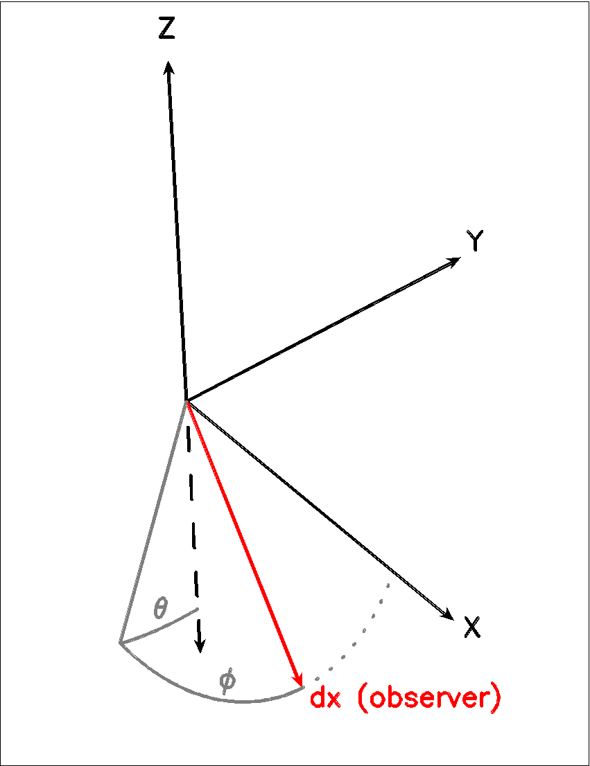
Fig. 1 The cartesian coordinate system used by LIME, showing the direction of the observer (red arrow) and the relation to the axes of the user-specifiable angles theta and phi.
Image rotation parameters
There are now two ways to specify the desired orientation of the model at the raytracing step: we have retained the old theta/phi angles, but have now added a new triplet: azimuth/inclination/PA. None of these five parameters is now mandatory. If none are provided, theta=phi=0 will be assumed. If you provide all three azimuth/inclination/PA values, these will be used instead of theta/phi, regardless if you also set either or both of theta/phi.
Note that all of these angles should be given in radians. You can however use the predefined PI macro for this: e.g. to express π/2, write PI/2.0 in your model file.
The rotation parameters in detail:
(double) img[i]->theta (optional)
Theta is the vertical viewing angle (the vertical angle between the model z axis and the ray-tracer’s line of sight). A face-on view (of models where this term is applicable) is 0 and edge-on view is π/2. The default value is 0.
(double) img[i]->phi (optional)
Phi is the horizontal viewing angle (the horizontal angle between the model z axis and the ray-tracer’s line of sight). A face-on view (of models where this term is applicable) is 0 and edge-on view is π/2. The default value is 0.
If theta/phi are applied, for zero values of both the model X axis points to the left, Y points upward and Z points in the direction of gaze of the observer (i.e. away from the observer).
(double) img[i]->azimuth (optional)
Azimuth rotates the model from Y towards X.
(double) img[i]->incl (optional)
Inclination rotates the model from Z towards X.
(double) img[i]->posang (optional)
Position angle rotates the model from Y towards X.
If azimuth/incl/posang are applied (i.e. if all three values are supplied in your model file), for zero values of all the model X axis points downward, Y points toward the right and Z towards the observer.
Model functions
The second part of the model file contains the actual model description. This is provided as eight subroutines: density, molecular abundance, temperature, systematic velocities, random velocities, magnetic field, gas-to-dust ratio, and grid-point number density. The user only needs to provide the functions that are relevant to a particular model, e.g., for continuum images only, the user need not include the abundance function or any of the velocity functions. The magnetic field function needs only be included for continuum polarization images.
Note that you should avoid singularities in these functions - i.e., places where LIME might attempt to divide by zero, or in some other way generate an overflow.
Density
The density subroutine contains a user-defined description of the 3D density profile of the collision partner(s).
void
density(double x, double y, double z, double *density){
  density[0] = f(x,y,z);
  density[1] = f(x,y,z);
  ...
  density[n] = f(x,y,z);
}
LIME can at present deal with 20 collision partners (CPs). (Note that there are only 7 listed in the LAMDA database.) In most cases, a single density profile will suffice. Note that the number of returned density function values no longer has to be the same as the number of CPs listed in the moldata file(s) so long as the user sets values for the collPartIds parameter; but if this parameter is not supplied, and the numbers are different, LIME may not be able to match the CPs associated with each density value to those in the moldata file(s). Note also that moldata CPs for which there is no matching density will be ignored.
The density is a number density, that is, the number of molecules of the respective CP per unit volume (in cubic meters, not cubic centimeters).
Molecular abundance
The abundance subroutine contains descriptions of the molecular abundance profiles of the radiating species in the input model. The number of abundance profiles should match exactly the number of molecular data files defined in par->moldatfile.
void
abundance(double x, double y, double z, double *abundance){
  abundance[0] = f0(x,y,z);
  abundance[1] = f1(x,y,z);
  ...
  abundance[n] = fn(x,y,z);
}
The abundance is the fractional abundance with respect to a weighted sum of the densities supplied for the collision partners. If the user does not supply the weights via the nMolWeights parameter, the code will try to guess them.
Abundances are dimensionless.
Molecular number density
As an alternative to the abundance function, the user is now able to supply a function which specifies directly the number density of each of the radiating species.
void
molNumDensity(double x, double y, double z, double *nmol){
  nmol[0] = f0(x,y,z);
  nmol[1] = f1(x,y,z);
  ...
  nmol[n] = fn(x,y,z);
}
The densities are number densities, that is, the number of molecules per unit volume (in cubic meters, not cubic centimeters).
Temperature
The temperature subroutine contains the descriptions of the gas, and optionally, the dust temperature.
void
temperature(double x, double y, double z, double *temperature){
  temperature[0] = f(x,y,z);
  temperature[1] = f(x,y,z);
}
The entry 0 in the temperature array is the kinetic gas temperature. This value is required for LIME to run. The entry 1 is the optional dust temperature. Both are in Kelvin. If there is no explicit dust temperature given in the temperature subroutine, LIME will assume that the dust temperature equals the gas temperature.
Random velocities
This subroutine contains a scalar field which describes the velocity dispersion of the random macroscopic (i.e. turbulent) motions of the gas. When added in quadrature to the thermal Doppler broadening specific to each molecule, this number gives the Doppler b-parameter which is the 1/e half-width of the line profile. The doppler subroutine differs from the other model subroutine in that the return type is a scalar, and not an array. The doppler value should be given in m/s.
void
doppler(double x, double y, double z, double *doppler){
  *doppler = f(x,y,z);
}
Because the return type is a scalar, the asterisk in front of the variable name needs to be present. doppler[0] does not work.
Velocity field
The velocity field subroutine contains the systematic velocity field of the gas. The return type of this subroutine is a three component vector, with components for the x, y, and z axis.
void
velocity(double x, double y, double z, double *velocity){
  velocity[0] = f(x,y,z);
  velocity[1] = f(x,y,z);
  velocity[2] = f(x,y,z);
}
In LIME 1.7 the previous ‘spline’ estimation (which was actually a polynomial interpolation) of velocities along the links between grid points has been replaced by a simpler system in which the velocity is sampled at (currently 3) equally-spaced intervals along each link, as well as at the grid cells. These link values are stored and used to estimate the average line amplitude per link via an error-function lookup. Ideally we would not need to call the velocity function again, but would be able to restrict calls of it (as is the case with all the other functions) purely to the gridding section. However it is found that linear interpolation of velocity within Delaunay cells at the raytracing is insufficient to produce accurate images; thus velocity is still called during the raytracing. In the near future we will try a 2nd-order in-cell interpolation, and if that proves adequate, we will have succeeded in relegating velocity calls to the gridding section alone.
Magnetic field
This is an optional function which contains a description of the magnetic
field. The return type of this subroutine is a three component vector,
with components for the x, y, and z axis. The magnetic field only has an
effect for continuum polarization calculations, that is, if
par->polarization is set.
void
magfield(double x, double y, double z, double *B){
  B[0] = f(x,y,z);
  B[1] = f(x,y,z);
  B[2] = f(x,y,z);
}
Gas-to-dust ratio
The gas-to-dust ratio is an optional function which the user can choose to include in the model.c file. If this function is left out, LIME defaults to a dust-to-gas ratio of 100 everywhere. This number only has an effect if the continuum is included in the calculations.
void
gasIIdust(double x, double y, double z, double *gtd){
  *gtd = f(x,y,z);
}
Grid point number density
In LIME 1.5 and earlier, the number density of the random grid points was tied directly to the density of the first collision partner. The newly introduced function gridDensity now gives the user the ability to option this link and specify the grid point distribution as they please. Note that LIME defaults to the previous algorithm if the function is not supplied.
double
gridDensity(configInfo *par, double *r){
  double fracDensity;
  fracDensity = f(r);
  return fracDensity;
}
- Notes:
- The returned variable is a scalar.
- This is the only function which includes the input parameters among the arguments. You cannot write to these, they are only supplied so that you can use their values if you wish to.
- Note that
fracDensityis interpreted as a relative value. LIME will scale the integral of the gridDensity function to the desired number of internal points set by the user via the parameterpar->pIntensity. - If you leave
par->samplingAlgorithmat its default of 0, but wish nevertheless to define a non-default gridDensity function, be aware that these two algorithms are a poor match, since they are built on different assumptions. You will need to make sure thatgridDensity()returnsfracDensity=1for at least one location in the model space in this case. Functions without steps are also recommended forpar->samplingAlgorithm==0.
Other settings
A number of additional settings can be found in the file
<LIME base dir>/src/lime.h. These settings should in general not be changed
by the user, unless there is an explicit need to do so. A few of them
however could be useful to some users. The keyword silent which is by
default set to zero can be set to one. This will cause LIME to run
completely silent with no output to the screen at all. This can be
useful for running LIME in batch mode in the background.
Advanced setup
Standard use of LIME requires the user to formulate the model in the model functions described above as either an analytical expression or a look-up table of values. As input models increase in complexity however, analytical descriptions may no longer be possible and with model dimensionality higher than one, look-up tables become difficult to manage within the model.c functions. In the following we will explain how to use complex numerical models and pre-gridded models as input for LIME.
Using numerical input models
Numerical input model can roughly be divided into two groups: those where the model properties are described as cell averages and those where the model properties are described at cell nodes (see figure). In either case, LIME will send a coordinate to the model functions and expect a value back. It is then up to the user to write an interface that will look up the appropriate return value.
In the simplest case where the numerical model is described as cell averaged values, the user needs to loop through the cells and find the cell in which the LIME point falls and return the value of that particular cell. In the case where the model is described on cell nodes, the user must loop through the nodes to find the node which lies closest to the LIME point and return that node value. This approach obviously limits the LIME model smoothness to the input model resolution since all LIME points which fall within an input model grid cell (or within a certain distance from a grid node) get the same value. One way to get around this is to interpolate in the input grid, which in principle can be done in either case, although this may be highly non-trivial if the model is described on unstructured grid nodes or is of a dimensionality greater than one. An example of linear interpolation in a one dimensional table can be found in the example model.c file below.
In the special case where the input model is described on unstructured grid nodes (e.g., Smoothed Particle Hydrodynamics simulations) the input grid can be used directly in LIME. This requires the user to set the par->pregrid parameter.
If the user is more comfortable writing code in the FORTRAN language, it is possible to use the model subroutines as wrappers to call FORTRAN functions which then carry out any necessary calculations and return the values to model.c. This can be done the following way:
void
density(double x, double y, double z, double *density){
  fortransub_(&x, &y, &z, &density[0]);
}
SUBROUTINE fortransub(x,y,z,temp)
DOUBLE x,y,z,temp
temp=f(x,y,z)
RETURN
END
In order for this to work the file containing the FORTRAN function needs to be compiled by a FORTRAN compiler and the resulting object file needs to be linked with LIME. This only works if the linking is also done with the FORTRAN compiler, so some modification to the Makefile is needed. Notice that the underscore after the name of the FORTRAN subroutine in the C function call has to be present. Please note that the example above is untested and may need modification in order to work.
If the input model file consist of a table of values, for instance as when using the output of another code as input for LIME, the idea is look up the input grid point (or cell) which is closest to the LIME grid point in question (or for cell based tables, the cell in which the LIME point falls). The way to deal with this is to make a column formatted ascii file with the input model:
x_1 y_1 z_1   density_1   temperature_1   any_other_stuff_1   ...
x_2 y_2 z_2   density_2   temperature_2   any_other_stuff_2   ...
...
x_n y_n z_n   density_n   temperature_n   any_other_stuff_n   ...
The idea is to find the i’th entry in that list where minimum((x_i-x)2+(y_i-y)2+(z_i-z)2) is true, or in other words which entry in the list lies closest to a given LIME point (x,y,z). One way to solve this would be as follows (example in pseudocode)
density(x,y,z){
 mindist=very_large_number
 open("model_input_file",read)
 while not end-of-file{
   read_one_line(x_i,y_i,z_i,density_i,...)
   calculate distance from (x,y,z) to (x_i,y_i,z_i) == dist
   if dist < mindist then {
     mindist = dist
     bestdensity = density_i
   }
 }
 close(file)
 return bestdensity
}
and similarly for the temperature and other properties. This is potentially a slow process, opening and closing a file for every grid point. To speed up the process, it is useful to make the model columns available as arrays in model.c. This can be done by formatting the columns using proper C-syntax as arrays and putting them in a “header” file that can be included in model.c
int size=numer_of_lines_in_model_file;
double model_x[size]={x1,x2,...,xn};
double model_y[size]={y1,y2,...,yn};
double model_z[size]={z1,z2,...,zn};
double model_density[size]={density1,density2,...,densityn};
...
The pseudocode example from above now reads:
density(x,y,z){
 mindist=very_large_number
 for i from 0 to size by 1
   calculate distance from (x,y,z) to (model_x[i],model_y[i],model_z[i]) == dist
   if dist < mindist then {
     mindist = dist
     bestdensity = model_densiy[i]
   }
 }
 return bestdensity
}
RATRAN models as input for LIME
It is possible to use existing 1D or 2D model files from the RATRAN code in LIME. This is done with ratranInput() subroutine. The .mdl file has to comply with the RATRAN standard and the header (everything above the @ sign) of the file needs to be intact. The functions in model.c look like this
void
density(double x, double y, double z, double *density){
  density[0]=ratranInput("model.mdl", "nh", x,y,z)*1e6;
}
and
void
temperature(double x, double y, double z, double *temperature){
  temperature[0]=ratranInput("model.mdl", "te", x,y,z);
}
for the density and temperature respectively. Notice that the density is multiplied by 1e6 to convert the cgs units from RATRAN into LIMEs SI units. The calls to the subroutine for the doppler velocity, systemic velocity, dust temperature, and abundance are similar, using the appropriate keywords to identify the column in the RATRAN .mdl file. Since RATRAN uses molecular density and not abundance, the abundance function should read
void
abundance(double x, double y, double z, double *abundance){
  abundance[0]=ratranInput("model.mdl","nh",x,y,z)/ratranInput("model.mdl","nm", x,y,z);
}
Obviously it is possible to mix RATRAN input, that is, using different
.mdl files for the different functions. All parameters in model.c still
need to be set, ie., par->radius, even though this information is
contained in the RATRAN header. If the RATRAN grid is not
logarithmically spaced, it may be advantageous to set par->sampling=1.
Output from LIME
Besides the FITS images, which are the main output, LIME produces other output that can be used not only for diagnostics but also science results. This chapter describes the various output files and how to work with them.
The grid
Once the Delaunay grid has been created by LIME, a VTK file with the
grid and grid properties are written (if the parameter par->gridfile is
set, see chapter 2). The VTK (Visualization Tool Kit) format is a
formatted ascii file that are used to handle geometrical objects, in our
case an unstructured grid. VTK files can be read by several
visualization software packages. In particular we advocate the use of
paraview (http://www.paraview.org) which is an open source program
available for several platforms.
The grid file contains the (x,y,z)-coordinate of each grid point, as well as a reference to the neighbors of each grid point. From this information the Delaunay triangulation can be reconstructed. The file also holds three scalar fields and a vector field for the H2 density, temperature, molecular density and the velocity field. Other properties could be written out as well, but that will require the user to edit the write_VTK_unstructured_Points() function in grid.c.
Inspecting the grid using paraview can be a useful way to make sure that the model indeed behaves as expected. It makes for impressive visualizations that can be included in presentations. However, paraview does a poor job when it comes to publication quality plots.
Populations
The level populations are written out in a separate file if LIME is set
up to calculate the level populations, that is, if at least one
molecular data file is defined in model.c (and if the parameter
par->outputfile is set). Currently, LIME can only write out populations
from the first molecule (par->moldatfile[0]). The populations output
file contains the x, y, and z coordinates for each grid point as well as
the H2 density, temperature, and molecular density besides the level
populations. Contrary to the grid file, it does not, however, contain
information about the neighbors of the grid points and therefore, the
Delaunay triangulation cannot be reconstructed from this file (unless
the points are re-triangulated with qhull or a similar tool). The
information in the population file allows the user to plot projections
and slices of the model properties including the populations. This is
the best way to directly compare the LIME model and the result of the
excitation calculation with the results obtained by other codes. One
particularly interesting property to plot is the excitation temperature
which is obtained from the level populations. u and l refers to the upper and lower level and g are the statistical weights. Calculating the excitation temperature is the best way to check for masering in the model since the excitation temperature turns negative in the case of population inversion. If, and only if, the gas is in local thermodynamic equilibrium (LTE) the excitation temperature equals the kinetic temperature, so plotting the ratio of kinetic gas temperature to the excitation temperature gives a measure of the deviation from LTE.
Images
Image cubes are the main output from LIME. LIME produces model images in the FITS file format only.
Post-processing
In order to make direct comparisons between LIME models and observations, some kind of post-processing of the images will be needed in almost all cases. In this chapter we will give some hints and tricks to how this can be done using readily available software packages.
Convolution
In order to compare LIME results to single dish observations, the image cube needs to be convolved with a beam profile that corresponds to the instrument beam at the frequency in question. Before convolving am image it is important to make sure that the image is larger that the beam size and that the beam is resolved by the pixels (pixel size << beam size). The reason that the image needs to be bigger that the beam is to avoid artificial edge effects at the corners of the image. This is not very important if only the spectrum toward the center of the image is of interest, but if the image is being used as a model of a single dish map, edge effects become important. In general, it is recommended that the image is made large enough that the emission has dropped sufficiently close to zero at the edges of the image.
If the beam size is small, it may be an issue that the beam is not sufficiently resolved by pixels.This is important to make sure that structures that are picked up by the telescope beam is sufficiently sampled by the ray-tracer in LIME. In general it is a good idea to calculate the image in a considerably higher resolution than what is needed, because artifacts in the image that are due to the randomness of the grid are then smoothed out. In order to compare a convolved model spectrum to a single observed spectrum toward the source center, the spectrum at the center pixel should be used without additional averaging of pixels.
When comparing model images to interferometric observations, there is no need to convolve the image with a beam profile. In this case, model and data is compared in frequency space in which case the model image needs to be Fourier transformed or in image space in which case the model should be sampled with the (u,v)-spacing from the dataset and inverted and cleaned using the same process as the observed data has gone through. When Fourier transforming the model image, one should be careful to avoid aliasing effects that are caused by the regularity of the pixel grid. Such effects are model dependent and difficult to prevent entirely. On the other hand, comparing the model to interferometric data in image space is dangerous as well, because of the non-uniqueness of the de-convolved image.
Both convolution and Fourier transforming can be done using the MIRIAD tasks convolve and fft after converting the FITS file into MIRIAD format using the MIRIAD task fits. Both convolution and Fourier transformation can be done in IDL or Python.
Plotting the model
The LIME data cubes can be visualized in numerous ways, both in one and two dimensions. One dimensional plots include the spectrum of a single pixel and the brightness profile along either spatial direction a a specific frequency or summed over a range of frequencies. The two dimensional (contour) plots are images when done in the plane spanned by the two spatial axis, and position-velocity (PV) diagrams when done in the frequency and any one of the spatial axis.
When plotting images, it is often useful to sum over a range of frequencies. This results in, what is know as, moment maps. These can be made to any order, but zero and first moments are most often used. The nth moment is defined as
Sometimes the first moment (and also higher order moments) is normalized by the zero moment.
Converting between old and new grid formats
Since LIME 1.7 the user has been able to store grid information corresponding to a number of different stages of processing in FITS-format files. This facility has been improved and tidied up for version 1.8; an HDF5 alternative has also been provided. Since the early days of LIME however the program has offered two ways to read in at least partial grid information, activated respectively by the parameters par.pregrid and par.restart. These pathways have been entirely superseded by the comprehensive FITS/HDF5 implementation but have been retained for the present to support backward compatibility. Be warned however that we intend eventually to dispense with them. To prepare for this situation, a new utility has been added to the LIME package: gridconvert. You will need to compile this yourself as a one-off, since no run-time compilation script is provided. Viz:
cd <LIME root directory>
make gridconvert
On the make line you can include the additional argument USEHDF5=yes if you prefer write/read to/from HDF5 instead of FITS. To clean up object files and other junk afterwards, do
make objclean
To clean everything away and restore the package to its status at download, do
make distclean
Running LIME in the usual way will not delete or otherwise affect gridconvert.
Ideas for LIME 2.0
In the following we list a number of new features which are being considered for the next major release of LIME. Users should feel free to contact the maintainers with suggestions, improvements, new functionalities or bugs needing to be fixed.
- Line polarization
- Visibility output
- Tau images
- User-defined, function based grid sample weights
- Basecol/Vamdc support
- etc…
Appendix: Bibliography
- Ade et al., A&A 576, A105 (2015)
- Bensch & Bergin, ApJ, 615, 531, 2004
- Brinch & Hogerheijde, A&A, 523, A25, 2010; see also http://www.nbi.dk/~brinch/lime.php
- Hogerheijde & van der Tak, A&A, 362,697, 2000
- Ritzerveld & Icke, PhysRevE, 74, 26704, 2006
- Ossenkopf & Henning, A&A, 291, 943, 1994
- Kernighan & Ritchie, “The C Programming Language 2nd ed.”, Prentice Hall, 1988, ISBN-13: 978-0131103627
- Padovani et al., A&A, 543, A16, 2012